第4章 Matlab 简易使用(二)
本期教程主要是讲解Matlab的简易使用方法,有些内容跟上一节相同,但是比上一些更详细。
4.1 Matlab的脚本文件.m的使用
4.2 Matlab中的条件和循环函数
4.3 绘图功能
4.4 总结
4.1 Matlab的脚本文件.m的使用
在matlab上创建和使用.m文件跟在MDK或者IAR上面创建和使用.C或者.ASM文件是一样的。创建方法如下:
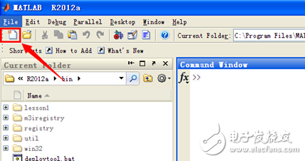
点击上图中的小图标,打开编辑窗口后,输入以下函数:
- % Generate random data from a uniform distribution
- % and calculate the mean. Plot the data and the mean.
-
- n = 50; % 50 data points
- r = rand(n,1);
- plot(r)
-
- Draw a line from (0,m) to (n,m)
- m = mean(r);
- hold on
- plot([0,n],[m,m])
- hold off
- title('Mean of Random Uniform Data')
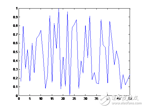
编辑好函数后需要将当前文件进行保存,点击File—>Save as即可,然后点击如下图标即可运行(或者按F5):

显示效果如下:
4.2 Matlab中的条件和循环函数
matlab也支持类似C语言中的条件和循环语句:for,while, if, switch。但在matlab中使用比在C中使用更加随意。
l 比如在.M文件中输入以下函数:
- nsamples = 5;
- npoints = 50;
-
- for k = 1:nsamples
- currentData = rand(npoints,1);
- sampleMean(k) = mean(currentData);
- end
- overallMean = mean(sampleMean)
在命令窗口得到输出结果:
- >> Untitled2 %这个是保存的文件名,运行相应文件会自动打印出
-
- overallMean =
-
- 0.4477
l 为了将上面函数每次迭代的结果都进行输出可以采用如下方法:
- for k = 1:nsamples
- iterationString = ['Iteration #',int2str(k)];
- disp(iterationString) %注意这里没有分号,这样才能保证会在命令窗口输出结果
- currentData = rand(npoints,1);
- sampleMean(k) = mean(currentData) %注意这里没有分号
- end
- overallMean = mean(sampleMean) %注意这里没有分号
在命令窗口得到输出结果:
- >> Untitled2
- Iteration #1
- sampleMean =
- 0.4899 0.4642 0.5447 0.4808 0.4758
-
- Iteration #2
- sampleMean =
- 0.4899 0.4959 0.5447 0.4808 0.4758
-
- Iteration #3
- sampleMean =
- 0.4899 0.4959 0.4977 0.4808 0.4758
-
- Iteration #4
- sampleMean =
- 0.4899 0.4959 0.4977 0.5044 0.4758
-
- Iteration #5
- sampleMean =
- 0.4899 0.4959 0.4977 0.5044 0.5698
-
- overallMean =
- 0.5115
l 如果在上面的函数下面加上如下语句:
- if overallMean < .49
- disp('Mean is less than expected')
- elseif overallMean > .51
- disp('Mean is greater than expected')
- else
- disp('Mean is within the expected range')
- end
命令窗口输出结果如下:
- overallMean = %这里仅列出了最后三行
- 0.5381
- Mean is greater than expected
4.3 绘图功能
4.3.1 基本的plot函数
l 根据plot不同的输入参数,主要有两种方式:
n plot(y),这种方式的话,主要是根据y的数据个数产生一个线性曲线。
n plot(x,y)以x轴为坐标进行绘制。
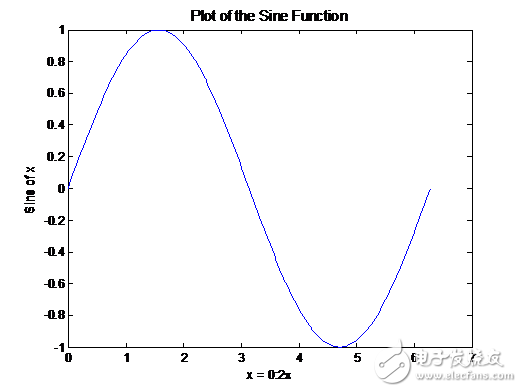
比如在命令窗口或者.m文件中写如下函数:
x = 0:pi/100:2*pi;
y = sin(x);
plot(x,y)
xlabel('x = 0:2\pi')
ylabel('Sine of x')
title('Plot of the Sine Function','FontSize',12)
l 下面这个函数可以实现在一个图片上显示多个曲线。
x = 0:pi/100:2*pi;
y = sin(x);
y2 = sin(x-.25);
y3 = sin(x-.5);
plot(x,y,x,y2,x,y3)
legend('sin(x)','sin(x-.25)','sin(x-.5)')

l 另外曲线的样式和颜色都可以进行配置的,命令格式如下:
plot(x, y, 'color_style_marker')

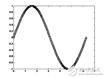
下面通过几个实例看一下实际显示效果。
x = 0:pi/100:2*pi;
y = sin(x);
plot(x,y,'ks')
显示效果如下:
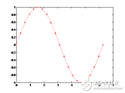
下面函数的显示效果:
x = 0:pi/100:2*pi;
y = sin(x);
plot(x,y,'r:+')

下面函数的显示效果如下:
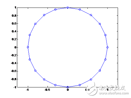
l 复数绘图
默认情况下函数plot只绘制数据的实部,如果是下面这种形式,实部和虚部都会进行绘制。plot(Z)也就是plot(real(Z),imag(Z))。下面我们在命令窗口中实现如下函数功能:
t = 0:pi/10:2*pi;
plot(exp(i*t),'-o')
axis equal
显示效果如下:
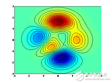
l 在当前的绘图中添加新的plot函数
使用函数holdon即可实现,这个函数我们在上一期中已经使用过,作用就是在当前绘图的基础上加上一个新的绘图。
- % Obtain data from evaluating peaks function
- [x,y,z] = peaks;
- % Create pseudocolor plot
- pcolor(x,y,z)
- % Remove edge lines a smooth colors
- shading interp
- % Hold the current graph
- hold on
- % Add the contour graph to the pcolor graph
- contour(x,y,z,20,'k')
- % Return to default
- hold off
显示效果如下:
l Axis设置
n 可见性设置
axis on %设置可见
axis off %设置不可见
n 网格线设置
grid on %设置可见
grid off %设置不可见
n 长宽比设置
axis square %设置X,Y轴等长
axis equal %设置X,Y相同的递增。
axis auto normal %设置自动模式。
n 设置轴界限
axis([xmin xmaxymin ymax]) %二维
axis([xmin xmaxymin ymax zmin zmax]) %三维
axis auto %设置自动
4.3.2 绘制图像数据
下面通过一个简单的实例说明一下图像数据的绘制,在命令窗口下操作即可。
>> load durer
>> whos
Name Size Bytes Class Attributes
X 648x509 2638656 double
ans 648x509 2638656 double
caption 2x28 112 char
map 128x3 3072 double
>> image(X) %显示图片

>>colormap(map) %上色

>> axis image %设置坐标

使用相同的方法,大家可以加载图片detail进行操作。另外用户可以使用函数imwrite和imread操作标准的JPEG,BMP,TIFF等类型的图片。
4.4 总结
本期主要跟大家讲解了Matlab的简单使用方法,后面复杂的使用需要大家多查手册,多练习。